- Examples
User Tools
Sidebar
Table of Contents
Optim user guide
Lagamine Inverse
The Lagamine Inverse code allows the computation of parameter sensitivity through a semi-analytical calculation. This implementation does not fundamentally change the code, but the simulation with Lagamine Inverse will be made so as to obtain both a reference finite element curve and the derivative of this curve with respect to the specified parameters.
To compute the derivative of the curve with respect to parameters, Lagamine will run one reference simulation with the input parameters and 2 additional simulations for each optimized parameter: one with a positive and on with a negative perturbation applied to the parameter (see OPTIM Description).
The values of the reference curve and its derivatives are put in a *.sm file at each iteration. When the Lagamine Inverse is used, the parameters specified by the user in the *.ia file are not read from the *.lag file but from the *.op file.
In order to launch a simulation using the Lagamine Inverse, several things are necessary:
- Modification of the IOPT parameter in the loading file *ex.dat;
- Implementation in the Lagamine subroutines INVA.F and WSENSM.F to specify the finite element curves to use;
Activation of Lagamine Inverse
In the *ex.dat file, the parameter IOPT (ninth parameter on the first line) must be set to 1 to activate the Lagamine Inverse simulation. It is also necessary to indicate an IDENT (5th parameter of first line) that allows the user to specify his curve in INVA.F and WSENSM.F (see figure 1). For the list of existing IDENT, see this page.
 Fig. 1: Example of *ex.dat file with activation of Lagamine Inverse
Implementation of the curves in INVA.F
The user must implement in the INVA.F subroutine the finite element curves that will be compared with the experimental curves (for instance, a stress-strain curve).
For each time step, subroutine INVA.F is called once for the reference simulation (ISENS=0), and twice for each optimized parameter (ISENS=1 for positive perturbation, ISENS=2 for negative perturbation). This allows to compute for every case the wanted curves $REACTION$ (reference), $REACTION_P$ (positive perturbation), $REACTION_M$ (negative perturbation). The computation of the sensitivity is then done according to the following:
\[DUef_{DX}(I,ILI)=\frac{REACTION_P(I)-REACTION_M(I)}{2*PREC_{IA} *XIAPAR(III,LLL)}\]
Where:
- $DUef_{DX}(I,ILI)$ is the derivatives of the Ith curve with respect to parameter n° $ILI$ (with $ILI=1,NBPAR_{OP}$)
- $REACTION_P(I)$ is the value of the Ith curve with a positive perturbation $PREC_{IA}*XIAPAR(III,LLL)$ on parameter n°$ILI$
- $REACTION_M(I)$ is the value of the Ith curve with a negative perturbation $PREC_{IA}*XIAPAR(III,LLL)$ on parameter n°$ILI$
- $PREC_{IA}$ is the relative perturbation
- $XIAPAR(III,LLL)$ is the value of parameter n°$LLL$ of law n°$III$ to be optimized
4 zones must be modified in the INVA.F subroutine to implement the computation of each reaction and of the derivative. These 4 zones are indicated by comments in the subroutine. Users must implement their curve using their IDENT number.
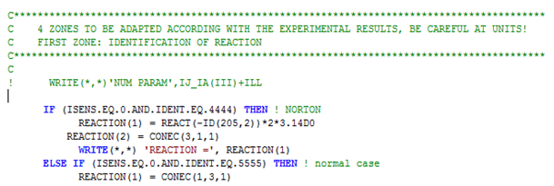
The first zone is used for the definition of the reference curves ($REACTION(I)$). It is necessary to write an “IF” condition imposing the chosen IDENT and ISENS=0. Users can then define as many curves as they want. The curves are taken from either nodal values (CONEC matrix), from integration point values (SIGVA vector), or from nodal reactions (vector REACT(-ID(Node, DOF))).
 Fig. 2: First zone to modify in the INVA.F subroutine
In the case shown in figure 2 with IDENT=4444, the first curve $REACTION(1)$ corresponds to the compression force on a cylinder. The reaction on DOF 2 (Y-direction) at node 205 is the reaction at the pilot node of the foundation in the axisymmetric case; this reaction multiplied by $2\pi$ gives the compression reaction on the cylinder. The second curve, $REACTION(2)$, is the coordinate of DOF 1 (X-direction) of node 3 at the end of the time step.
The second and third zones are used for the implementation of the perturbed curves. The second zone is for the positive perturbation ($REACTION_P$) while the third is for negative perturbation ($REACTION_M$). In these cases, matrices CONEC and SIGVA must be replaced respectively by CONEC_PERT_P or CONEC_PERT_M, and SIGVA_PERT_P or SIGVA_PERT_M.
 Fig. 3: Second zone to modify in the INVA.F subroutine
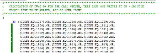
The fourth zone is for the computation of $DUef_{DX}(I,ILI)$. This calculation is already defined in the code, users simply need to add their IDENT number in the “IF” list as shown in figure 4.
 Fig. 4: Fourth zone of the INVA.F subroutine
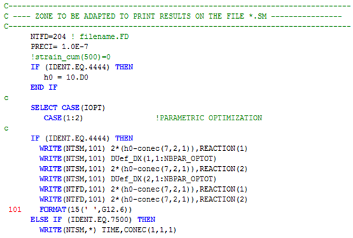
Implementation of the printing in WSENSM.F
The results computed in INVA.F at each time step are then sent to the WSENSM.F subroutine to be printed in a *.sm file and in a *.fd file. The *.sm file contains the values of the curves and their derivatives for every time step and is used by Optim to compute the objective function and its derivative. The *.fd file only contains the finite element curves and can be used to easily visualize results in postprocessing.
Similarly to the INVA.F subroutine, users must indicate their IDENT in an “IF” condition. Then, the printing in the *.sm file (ntsm)must be defined as follows:
- On the first line, write the abscissa and ordinates (REACTION(1)) of the first curve;
- On the second line, write the derivatives of this curve with respect to the parameters;
- If there are more than one curve, repeat line 1 and 2 for REACTION(I)
Afterwards, the curves can be printed in the *.fd file (ntfd)
Example:
  if(IDENT.EQ.XXXX) then
      write(ntsm,*) abscissa, reaction(1)
      write(ntsm,*) DUeF_DX(1,NBPAR_OPTOT)
      write(ntsm,*) abscissa, reaction(2)
      write(ntsm,*) DUeF_DX(2,NBPAR_OPTOT)
      write(ntfd,*) abscissa, reaction(1)
      write(ntfd,*) abscissa, reaction(2)
  endif
The example for IDENT=4444 is illustrated in figure 4, where the abscissa corresponds to the height of the cylinder during the compression loading.
 Fig. 5
Files
To launch a simulation with Lagamine Inverse (even without using Optim), specific files *.op and *.ia are required to define which parameters are optimized. The description of these files can be found here.
Optim
To launch an optimization with Optim, several files are required:
- Lagamine simulation files *.lag and *ex.dat;
- Definition of the optimized parameter initial values *.op;
- Definition of the number of curves and parameters to be optimized *.ia;
- Definition of the experimental curve(s) *.exp;
- Main input for Optim *.info.
The structure of these files is detailed in the File section of this manual.
Structure of the code
The code Optim is structured in several subroutines:
- Main_levenberg: reading of files *.ia, *.op, *.exp and *.info + initialization of variables;
- pre_optim: initialization of optimization parameters;
- algo_leven: Levenberg-Marquardt algorithm;
- fcn: execution of Lagamine Inverse simulation, interpolation of the curves at points i=1,NPOI, computation of fvec vector containing the residuals at each point;
- fdjac: interpolation of the derivatives and computation of matrix fdjac containing the derivative of the curves at points i.
The algorithm can be summed up as follows:
- MAIN_LEVENBERG
Read *.info file, *.exp file, *.op file
Run prepro
Initialize variables and allocate memory
Call PRE_OPTIM- PRE_OPTIM
Check input parameters
Initialize Optim parameters
Call ALGO_LEVEN- ALGO_LEVEN
Check input parameters
Call:- FCN
Launch Lagamine simulation
Read *.sm file
Compute EF and REF curves - ENORM
Compute the norm (objective function) - FDJAC
Compute sensitivity matrix (Jacobian) from *.sm file - QRFAC
QR factorization of the Jacobian - LMPAR
Determine Levenberg-Marcquardt parameters
- Check for convergence
If no → loop
If yes → end
Files used by Optim
| Type | Unit | Description |
|---|---|---|
| .exp | 1 | Experimental (reference) curve |
| .info.FPA | 2 | Recording of every optimization step (parameters + norm) |
| .fd | 8 | Result from Lagamine Inverse |
| NFEV.fd | 9 | Result from Lagamine Inverse at iteration NFEV |
| .sm | 10 | Result from Lagamine Inverse |
| ex.dat | 11 | Loading file for Lagamine |
| FCT_OBJECTIF.OPT | 12 | Result file |
| .op | 13 | Parameters to be optimized |
| .ia | 20 | Input data for Lagamine Inverse |
| .info | 78 | Input data for the optimization |
| fvec.vm | 88 | Record difference between EF curve and REF curve |
Results and output files
During the optimization, the intermediary results are printed out in the console window as well as in the *info.FPA file.
When the objective function is reduced, the result and the corresponding parameters are written in the FCT_OBJECTIF.OPT file.
